Basic HTML Version


224
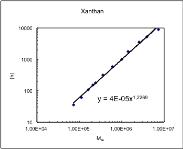
Thus, a plot of log
[η]
versus log M should – for a given polymer system –
give a straight line where the shape-dependent exponent (a) appears as the
slope (Fig. 11.7 in textbook). The example below shows literature data
44
for
xanthan fractions (carefully prepared by degradation and fractionation).
The figure is a double-logarithmic plot with geometric fitting, which is
equivalent to a linear plot after talking logarithms and performing a linear
regression, providing the exponent a (1.23) directly, or as slope, respectively.
The value shows xanthan behave somewhat between a rigid rod (1=1.8) and
a random coil.
Here is another example, showing
[η]
-M data for chitosans and lignosulfonate
(data obtained at NOBIPOL):
The chitosans behave as randomly coiled polymers in a good solvent (Acetate
buffer pH 4.5. Why not pH 7?) with a MHS exponent of 0.88. In contrast,
44
- Sato et al., Macromolecules, 17 (1984)
y =
0.010x
0.883
y =
0.121x
0.358
1
10
100
1,000
10,000
1,000
10,000
100,000
1,000,000
M
w
(acetate) (SEC-
[h] (recalculated as acetate) (ml/g)